Lab 3: Introduction to Python I

Lab 3: Introduction to Python I#

In this class, we will be using Python for data analysis and visualization.

To run the lab interactively, click the Binder button below:

Why Use Python?#

General-purpose, cross-platform
Free and open source
Users can quickly learn how to do basic tasks
Robust ecosystem of scientific libraries, including powerful statistical and visualization packages
Large community of scientific users and large existing codebases
Major investment into Python ecosystem by Earth science research agencies, including NASA, NCAR, UK Met Office, and Lamont-Doherty Earth Observatory. For example, see Pangeo.

Lesson Objectives#

You will learn:
- The basics of using Jupyter Notebook
- Basic syntax of Python
- Data types, lists, and arrays
- Reading in ASCII data
- Filter data and calculate basic summary statistics
- Basic plotting and visualization

Using Jupyter Notebook for Python#

A Jupyter notebook allows you to easily run Python commands and check the output interactively. To run your Python code, type the code into a cell, highlight the cell, and either click the run button (►) or press the Shift and Enter keys.

Adding comments to your code is an important habit and essential for documenting and sharing work, so let’s start doing that now.

# This is a comment, meant for a human. Python ignores it.
print("Hello MAS 331L!")

Hello MAS 331L!

A computer is a really big calculator. You can use Python in this notebook just like a calculator. What’s one plus one?

#Do you need a comment here?  Maybe not, but do it anyway as good practice.
1+1

Here are some of Python’s built in mathematical operators, and some commands you can run in the next cells.

Operator	Syntax	Commands to run in the next cells
Addition	+	6 + 2.0
Subtraction	-	3 - 1
Multiplication	*	2.8 * 82
Division	/	57 / 3
Exponential	**	2 ** 3
Integer Division	//	5 // 2
Modulus	%	5 % 2

Exercise 1:

Try the following to learn the basics of using Jupyter Notebook.

Create a few new cells, some by using the menu and some with key commands. (Hint: Insert, A, B)
Figure out how to delete a cell using the menu or keyboard. (Hint: Edit, DD)
Create new cells and try all of the commands above.
Create a new cell and change it to Markdown, which is what I am using to type these instructions. Say hello.

#I just added a Code cell...your turn for the rest
6 + 2.0

8.0

Saving your work#

Save your progress periodically by clicking the disk icon or selecting File : Save Notebook. Closing Binder will delete all of our data.

At the end of class, you will download your notebook with the completed exercises and turn it in as the lab assignment.

If you’d like, you can periodically save a copy to your local machine by doing File : Download. This lab is not expected to crash, but anything is possible. If you will try operations not covered in the notebook, we recommend that you download the notebook before doing so.

One more troubleshooting item:

If you run a cell and nothing happens, check the top right-hand corner of the notebook. Binder ‘turns off’ or pauses our computer if it is idle or if something goes wrong. If you see No Kernel, click ‘No Kernel’ and click the Select button in the popup window.

Acknowledge the Following

Acknowledge that you understand the significance of ephemeral data, the procedure for submitting the lab assignment, and the requirement to comment code by cutting and pasting each of the following into the next three cells

#I understand that Binder will delete all of my data when I exit the notebook
#I understand that after completing the exercises, I need to save a copy of the notebook to my local machine to submit as the lab assignment
#I understand that I am expected to comment my code.

Variables#

A variable stores a value. For example, here, c is a variable:

c = 299792458

Variable names can contain only letters, digits, and underscores, and they are case sensitive.

Choose variable names that actually describe the value they are holding. For example:

speed_of_light = 299792458

Intuitive variable names are key to writing clear, easy to read, reusable code.

Next: Define some variables!

#Define a bunch of variables!
var_int    = 8
var_float  = 15.0
var_4e8    = 4e8
var_string = 'Hello MAS 331L!'

Defining a variable will not return any output. Add print statements to check values within a block of code.

Exercise 3:

Fill in the next cell using print statements.

#Add print statements to check the variables you set above.  
#I'll do the first one, and you add the rest.
print(var_int)
#Your turn
#

Types#

Every variable has a type. In some languages, the programmer has to declare the type before using the variable. For example, in C:

int   my_id
char  my_letter
float speed_of_light

Python is ‘dynamically typed’, which means that you don’t need to declare variables. Instead, Python will automatically guess the variable type based on what operations you are attempting to perform. That said, you should have an awareness of basic variable types.

Numbers
int - an integer is a whole number, positive or negative
float - a floating point number is a positive or negative number containing decimal digits
Characters
str - a string is a sequence of character data
Boolean
bool - a boolean is either True or False

To check the type of a variable, use the type() function. Print out the types for the variables you declared earlier.

#Print out the variable types
print(type(var_int))
print(type(var_float))
print(type(var_4e8))
print(type(var_string))

<class 'int'>
<class 'float'>
<class 'float'>
<class 'str'>

Functions#

Python has many built in functions, and the syntax is usually:

function_name(inputs)

We have already been using two functions: print() and type().

#Using functions print and type
print("Here comes a list of the types...")
type(var_int),  type(var_float), type(var_4e8), type(var_string)

Here comes a list of the types...

(int, float, float, str)

Exercise 4:

Use type() to test if the following are floats or integers:
- 2+2
- 2*2.0
- var_float/var_int
Try some mathematical operations on strings:
- “Hello MAS 331L!” + “Peace Out.”
- 4 * “Happy”
- 4 + “Happy”
Use a Markdown cell or a code comment to say which thing didn’t work and why.

Your Solutions:

Working with Lists#

Lists are useful for storing data. Lists are made using square brackets. They can hold any data type (integers, floats, and strings) and even mixtures of the two.

#Define a list of integers
numbers_list = [4, 8, 15, 16, 23]

You can access elements of the list using the index. Python is zero based, so index 0 retrieves the first element.

#Show the element with index 3
numbers_list[3]

New items can be appended to the list using the append function, which has the syntax:

variable.function(element(s))

The list will be updated in-place, which means the function will directly modify the list.

#Append a number to our list and show the result
numbers_list.append(42)
numbers_list

[4, 8, 15, 16, 23, 42]

Sometimes you would want to add the numbers in a list, element by element; however, the addition operator works differently on lists. For list objects, the + will combine lists. To perform mathematical operations, you must convert a list to an array using the NumPy package.

Exercise 5:

Confirm that numbers_list+numbers_list does not add list items element by element, but appends a copy of itself.
Try multiplying numbers_list by an integer number.
Show only the first 4 elements of numbers_list. The syntax for taking a subset of a list is [x:y].
Append your name to the list. A string has quotes, e.g. “Bob”. Display the resulting numbers_list. Did it work?

Your Solutions:

If you successfully added your name to our numbers_list, then it won’t be just numbers. Let’s fix it before using it as a numerical array in the next section.

#Reset our array so it contains only numbers
# or else it will give us errors in the next section
numbers_list = [4, 8, 15, 16, 23, 42]

Importing Packages#

Packages are collections of modules which help simplify common tasks. NumPy is essential for mathematical operations and array manipulation.

NumPy:

Creates high-performance multidimensional array objects and provides tools for working with these arrays.
Is a fundamental package for scientific computing with Python.
Is included with the Anaconda package manager.
For additional examples, please refer to the the NumPy Quick Start.

The basic syntax for importing packages is import [package name]. Some packages have long names. You can use import [package name] as [alias] to avoid repeatedly typing that long name.

#Import the NumPy package and call it 'np'
import numpy as np

If you do not see any error after running the line above, then the package was successfully imported. If you see an error, it probably means the package is not installed.

Working with Arrays#

I can use NumPy’s array constructor np.array() to convert our list to a NumPy array in order to perform mathematical array operations on it. For example, I can double each element of the array:

#Use NumPy to convert the list into an array
numbers_array = np.array(numbers_list)
#Show the result of multiplying by 2
numbers_array*2

array([ 8, 16, 30, 32, 46, 84])

Another difference between arrays and lists is that lists can only be one-dimensional. NumPy can be any number of dimensions. For example, I can change the dimensions of the data using the reshape() function:

#Create a 2D array using the reshape function
numbers_array_2d = numbers_array.reshape(3,2)
#Display the result
numbers_array_2d

array([[ 4,  8],
       [15, 16],
       [23, 42]])

The shape attribute gives the dimensions of the new array.

#Display the dimensions of the new array.
numbers_array_2d.shape

(3, 2)

The original numbers_array had a length of 6, and the new array has 3 rows and 2 columns.

Exercise 6:

Create a longer list, called long_list, by multiplying numbers_list by 5.
Convert the list into a NumPy array, called long_array.
Reshape long_array into a 2D array.
Reshape long_array into a 3D array.

Note: For 3 and 4, you will get errors unless the dimensions are compatible with the original array length. Read the error and try again.

Your Solutions:

If you are having trouble with the above exercise, make sure numbers_list is set correctly, or just reset it here:

#If you are having problems, you may need to reset the numbers_list
numbers_list = [4, 8, 15, 16, 23, 42]

Why am I reshaping arrays??#

Just to introduce NumPy. Python will often return things as lists, and you can't perform mathematical operations on a list. NumPy can take whatever weird data object you've been stuck with and transform it into something you can do science with. NumPy mathematical functions are also lightning fast compared to the equivalent base Python funtions.

Reading ASCII Data#

The Pandas package has a function for reading text/ASCII data called read_csv(). Although the function appears to be meant for reading CSV files, read_csv will read any delimited data using the sep=* keyword argument. Below, you will import the Pandas package and read in a dataset. Note that the path below is relative to the current notebook and you may have to change the code if you are running in a different environment.

data/MB8J.csv

We will look at a data file containing daily temperature and salinity data.

#Import Pandas and alias it as 'pd'
import pandas as pd

This actually is a properly formatted CSV file, so the sep=',' is not technically required. The engine='python' ensures that the command will work across different operating systems.

#Defining the filename allows you to write code that can be reused with different files
filename = "data/MB8J.csv"
#Although not descriptive, df is used in R and Python for data frames 
# because it is short and will need be used and reused often during data cleaning
df = pd.read_csv(filename, sep=',', engine='python')

You can inspect the contents of the dataset using the head() function, which will return the first five rows of the dataset. Pandas automatically stores data in structures called DataFrames. DataFrames are two dimensional (rows and columns) and resemble a spreadsheet. The leftmost column is the row index and is not part of the dataset.

#Peek at the data
df.head()

	CTD	Date	T-Surface	T-Bottom	S-Surface	S-Bottom
0	MB8J	1/1/2019	19.418117	19.323412	8.746278	11.118851
1	NaN	1/2/2019	19.752113	19.416435	8.018461	11.788327
2	NaN	1/3/2019	19.865190	19.771955	10.140968	11.814590
3	NaN	1/4/2019	19.204679	19.229073	11.242235	11.247988
4	NaN	1/5/2019	16.833044	17.105726	8.877601	11.490634

The data contains a time series of bottom and surface temperature and salinity. The column CTD has the name of the station in the first row, followed by nothing. If you look in the original file with Excel, each row under MB8J is empty. Empty cells are labeled NaN - Not a Number.

You can extract a specific variable from the dataset by using the column name. This is the time to choose a more descriptive variable name. Let’s extract the surface temperature and look at the first five rows.

#Get the surface temperature and check the values
temp_surf = df['T-Surface']
temp_surf.head()

  19.418117
  19.752113
  19.865190
  19.204679
  16.833044
Name: T-Surface, dtype: float64

Now that we have an array of numbers, we can do general statistics on it. Check the min, max, and mean of the data.

#Find min, max, and mean
temp_surf.min()
temp_surf.max()
temp_surf.mean()

24.135902121257146

Executing a block of code will only list the output of the last command, so we need to add some print statements. Also, these statistics might come in handy, so let’s save each of them to a variable.

#Save the statistics to variables
temp_surf_min = temp_surf.min()
temp_surf_max = temp_surf.max()
temp_surf_mean = temp_surf.mean()
#Print them out in a way that is useful and easy to read
print("Tmin =",temp_surf_min,", Tmax =",temp_surf_max,", Tmean =",temp_surf_mean)

Tmin = 11.32288893 , Tmax = 32.76987648 , Tmean = 24.135902121257146

Is it reasonable for Tmean to be written with such precision? Do you ever hear the weather forecast to eight decimals? Introducing the round() function. When you are working with data, keep measurement uncertainty in mind when doing the calculations, and keep readability in mind when writing a general report. So, as a new reporter for SeaTemperature.org, I might do:

#One decimal is good enough for my boss...
print("Surface Temperatures - Min:",round(temp_surf_min,1),"Max:",round(temp_surf_max,1),"Avg:",round(temp_surf_mean,1))

Surface Temperatures - Min: 11.3 Max: 32.8 Avg: 24.1

Exercise 7: Give a report on the bottom temperature

Get the bottom temperature and check the values
Find min, max, and mean, and save to variables
Print them out in a way that is useful and easy to read

Your Solutions:

Filtering data#

When working with data, you may want to remove outliers or focus on a specific location or date range. For example, you may only want examine data below or above a certain threshold. You can subset the data using comparison operators:

less than: <
less than or equal to: <=
greater than: >
greater than or equal to: >=
equals: ==
not equals: !=

A comparison espression returns a True or False statement. Here are some examples:

#True or False?
"Apples" == "Oranges"

False

#True or False?
500 <= 1

False

You can also use a comparison expression to define a variable. The data type is called a ‘boolean’, and boolean values are either True or False.

#True or False and what type?
fruit = "Apples" != "Oranges"
print(fruit)
print(type(fruit))

True
<class 'bool'>

Comparison expressions may be combined using and (&) and or (|).

#Is 5 greater than 1 but less than 10?
5 > 1 & 5 < 10

True

Our data has temperature and salinity. I don’t like to swim unless the water is nearly bathtub temperature, and I don’t care what the salinity is if I’m not swimming. I can limit my dataset by creating a conditional expression such that the temperature is over 31°C. We use this conditional expression to create what is known as a ‘mask’, which can be used later to create a new dataset with only the data we are interested in.

#Mask will be True for all values over 31
#Recall: temp_surf = df['T-Surface']
temp_mask = temp_surf  > 31
#Only the first 5 and last 5 rows of df are shown
print(temp_mask)

    False
    False
    False
    False
    False
       ...  
  False
  False
  False
  False
  False
Name: T-Surface, Length: 350, dtype: bool

Applying the mask to the original temperature dataset gives us the subset of temperature data we’re interested in.

#Just get the warmer water data
warm_data = temp_surf[temp_mask]
print(warm_data)

  31.002864
  31.302196
  31.704169
  31.421270
  31.217889
         ...    
  31.768182
  31.357623
  31.072324
  31.348356
  31.318060
Name: T-Surface, Length: 69, dtype: float64

How does my temperature preference affect the number of days I might go for a swim? Use the size attribute to find out.

#How often would I go swimming?
print("I would only go swimming on ", warm_data.size,"of the", temp_surf.size, "dates included in this dataset.")

I would only go swimming on  69 of the 350 dates included in this dataset.

Exercise 8: Your turn to filter some data

Starting from the original dataset df:

Create a mask that filters the surface temperature to ‘perfect pool’ temperatures (25 - 28°C). Hint: Put parentheses around your conditional expressions.
Apply your mask to the surface salinity taken from the original data set.
Find the average surface salinity for 1) the entire dataset and 2) the ‘perfect pool’ dataset.
Make a report summarizing your findings.

Your Solutions

Basic Figures and Plots#

For visualization with Python, folks use Matplotlib. Here is what Matplotlib has to say about itself:

Matplotlib is a comprehensive library for creating static, animated, and interactive visualizations in Python. Matplotlib makes easy things easy and hard things possible.

That sounds pretty good. Let’s try it out. First, import the package.

#import matplotlib, call it plt
import matplotlib.pyplot as plt

#And I forget what our data looks like... 
df.head()

	CTD	Date	T-Surface	T-Bottom	S-Surface	S-Bottom
0	MB8J	1/1/2019	19.418117	19.323412	8.746278	11.118851
1	NaN	1/2/2019	19.752113	19.416435	8.018461	11.788327
2	NaN	1/3/2019	19.865190	19.771955	10.140968	11.814590
3	NaN	1/4/2019	19.204679	19.229073	11.242235	11.247988
4	NaN	1/5/2019	16.833044	17.105726	8.877601	11.490634

Time series plots#

I have dates, and I have data. Matplotlib has a plot() function. If Matplotlib lives up to it’s hype, I can make a plot with no worries.

#Attempt a time series plot
plt.plot(df["Date"], df["T-Surface"])

[<matplotlib.lines.Line2D at 0x173d47d90>]

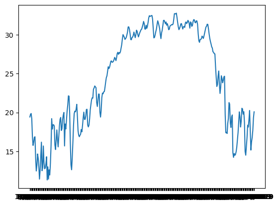
_images/a760a991183e05ffe69f47242655532092f0349fbfbe446f0a014297c27040c8.png

So it is relatively easy to get a plot. How about a decent looking plot? If you take a look at the axes, the y axis looks normal and the x axis looks like garbage. This is because of the date formatting. We’ll revisit date/time formatting in the next lab. First, let’s just try some simple formatting with other types of plots.

Histograms#

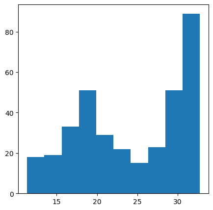
Let’s try a histogram, which shows a count of how many data points have a certain range of values. This time we will do some basic plot formatting.

In Matplotlib, we create a blank canvas, we paint whatever we want, and when we’re finished and ready, we show off our art. Here is the beginner painting.

plt.figure() creates a blank canvas with specified dimensions
plt.hist() adds the histogram
plt.show() completes and renders the plot

#Basic histogram of surface temperature
plt.figure(figsize=[5,5])
plt.hist(df["T-Surface"])
plt.show()

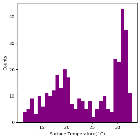
_images/dd3c71015c89ad65c9bdf75adfb19373527884be9f238ecbe5f005a1546cfdf4.png

For the next round, let’s modify by:

Giving the histogram a bin number instead of using the default
Changing the color of the histogram
Adding x and y labels

#Refined histogram of surface temperature with labels
plt.figure(figsize=[5,5])
plt.hist(df["T-Surface"],bins=30,color="purple")
#Google-search the special characters when you need them, like the degree symbol
plt.xlabel('Surface Temperature($^\circ$C)')
plt.ylabel('Counts')
plt.show()

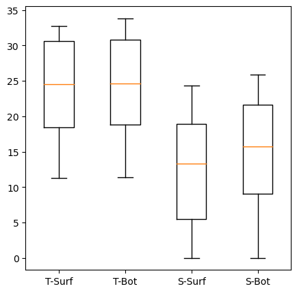
_images/a0e725780a46cb10dec56a7c7cf7b13e03c7755608f5cee6a4f2a77c5c56e32e.png

Box Plots#

Let’s try a box plot. A box plot, or box and whisker plot, displays the minimum, first quartile, median, third quartile, and maximum of a dataset. Sometimes it also displays the outliers.

I don’t like a lonely box plot, so let’s look at box plots of all the quantities. This is where a list comes in handy. Pass a list of the data to the boxplot function.

#Friendly box plots
plt.figure(figsize=[5,5])
#Create list of temperature data
list_of_data = [df["T-Surface"],df["T-Bottom"],df["S-Surface"],df["S-Bottom"]]
#And a list of labels
list_of_labels = ['T-Surf','T-Bot','S-Surf','S-Bot']
#Make the boxplots
plt.boxplot(list_of_data,labels=list_of_labels)
plt.show()

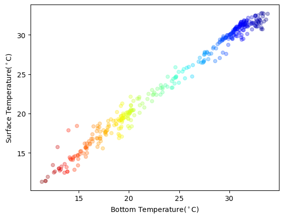
_images/fe0d67b207755f4a21ac7d0fd0252a6e48f23a017d00a8a6769bd02be5b84987.png

Scatter plots#

And the good ole’ scatter plot. Let’s make things interesting by adding a colormap.

In the next plot, we:

Import the colormap package.
Choose a colormap. This example chooses ‘Jet’, popular to the masses and discouraged by visualization gurus. Personally, I love rainbow dots.
Choose a variable to color by. Our colormap will change according to bottom temperature.
Create a scatterplot of surface and bottom temperatures.

In the scatterplot function:

plt.scatter(x, y, s, c, cmap, alpha)

x = data position
y = data position
s = marker size
c = sequence of numbers to be mapped to colors
cmap = colormap
alpha = transparency, where opaque==1

#import colormap package
import matplotlib.cm as cm

#variable to color by, and the name of our colormap
colorby = df['T-Bottom']
colormap = 'jet_r'

#Create a scatterplot of surface and bottom temperature and color by bottom temperature
#Use big dots and make the dots semi-transparent
plt.figure()
plt.scatter(df['T-Bottom'], df['T-Surface'], s=25, c=colorby, cmap=colormap, alpha=0.3)
plt.xlabel("Bottom Temperature($^\circ$C)")
plt.ylabel("Surface Temperature($^\circ$C)")
plt.show()

_images/aacb59d87ad0f25e2f1dd9b36c6d43258542bb42e80977faedca89a9c05b03aa.png

Exercise 9: Create your own plot.

Recreate any of the plots above, but use different variables, modify the labels, and change attributes such as colors or colormap.

Optional:

If you have time and interest, try any of the following with the help of Google or the Matplotlib documentation.

Choose custom limits for the x and y ranges.
Add a title.
Show multiple plots in one figure.
Try different colormaps, and read a bit about choosing colormaps for accessibility. See for example: Info on colorblindness and Python packages for choosing colormaps.
Make a timeseries plot with reasonable x-axis labels, or simply remove the x-axis labels completely. Add additional variables to the timeseries plot. Choose different colors or symbols (e.g., dotted, dashed, etc.) for the different variables, and create a legend.

Your Solution:

Turn in your lab#

Download your notebook with the completed exercises and turn it in as the lab assignment.

Summary:#

You have learned:
- The basics of using Jupyter Notebook
- Basic syntax of Python
- Data types, lists, and arrays
- Reading in ASCII data
- Filter data and calculate basic summary statistics
- Basic plotting and visualization

Attribution#

Creating this lab was facilitated by using content from AGU 2021 Python for Earth Sciences workshop, developed and led by Rebekah Esmaili (bekah@umd.edu), Research Scientist, STC/JPSS. We are grateful for Rebekah’s generous support of Open Science and sharing all her hard work!

Lab 3: Introduction to Python I

Contents

Lab 3: Introduction to Python I#

Why Use Python?#

Lesson Objectives#

Using Jupyter Notebook for Python#

Saving your work#

Variables#

Types#

Functions#

Working with Lists#

Importing Packages#

Working with Arrays#

Why am I reshaping arrays??#

Reading ASCII Data#

Filtering data#

Basic Figures and Plots#

Time series plots#

Histograms#

Box Plots#

Scatter plots#

Turn in your lab#

Summary:#

Attribution#